A tour of the UI
This tour walks through every screen of the OEDI-SI web app in the order you’ll use them, from the landing page to the analysis notebook. The screenshots use the built-in NLR DSSE IEEE 123 example — an IEEE 123-bus feeder feeding a measurement layer and a weighted-least-squares state estimator, with recorders capturing the results.
Home
The landing page is your hub. Each card is an entry point: create a new simulation, open a saved one, or check simulation status.
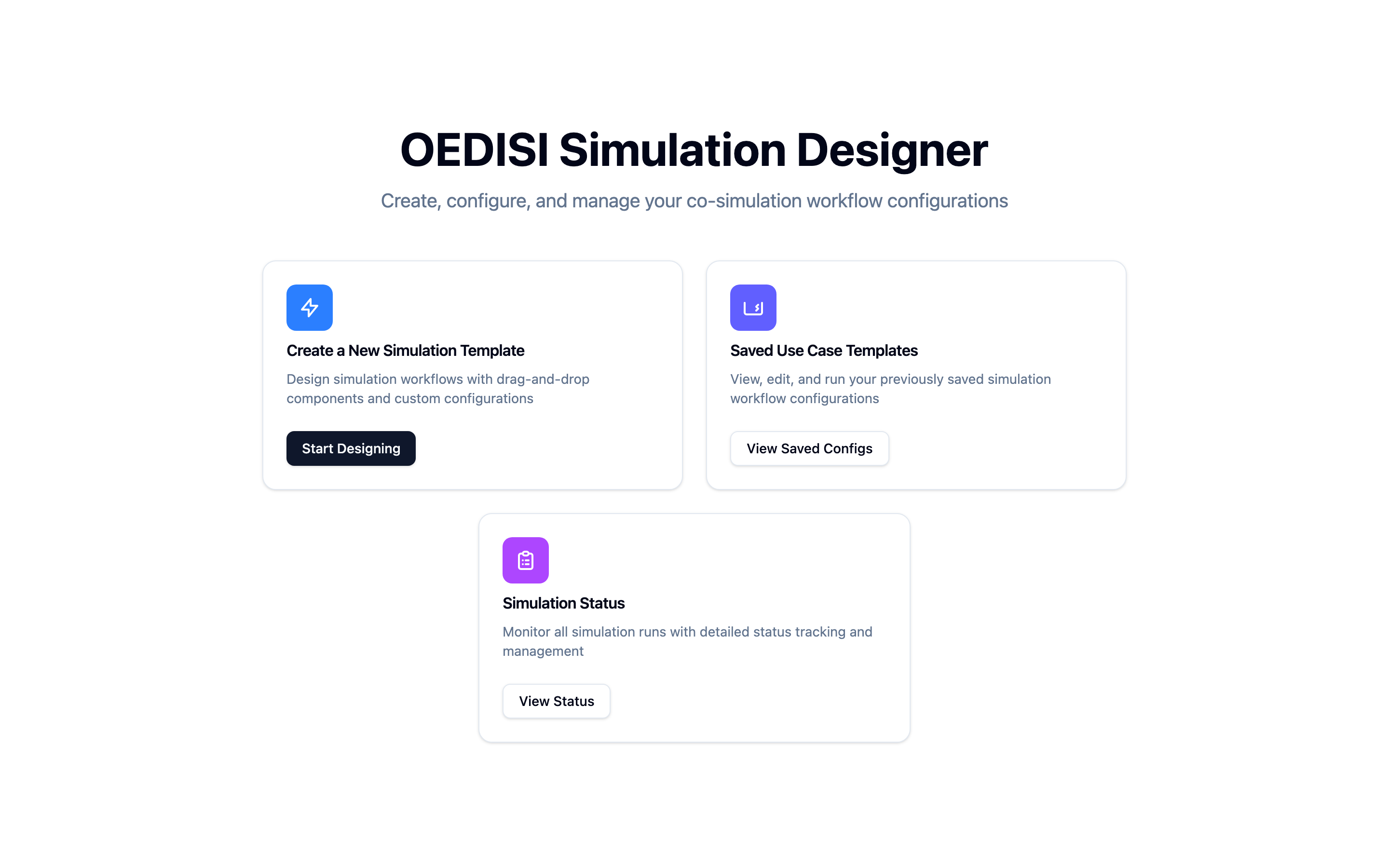
The OEDI-SI home page.
The designer
Start Designing opens the flowchart designer — where a simulation is assembled. It has three regions:
Components palette (left) — every registered component you can drag onto the canvas. See the full list in the component catalog.
Canvas (center) — the wiring diagram. Nodes are components; edges are typed connections between their ports.
Properties panel (right) — configure the selected component’s inputs, or inspect a connection.
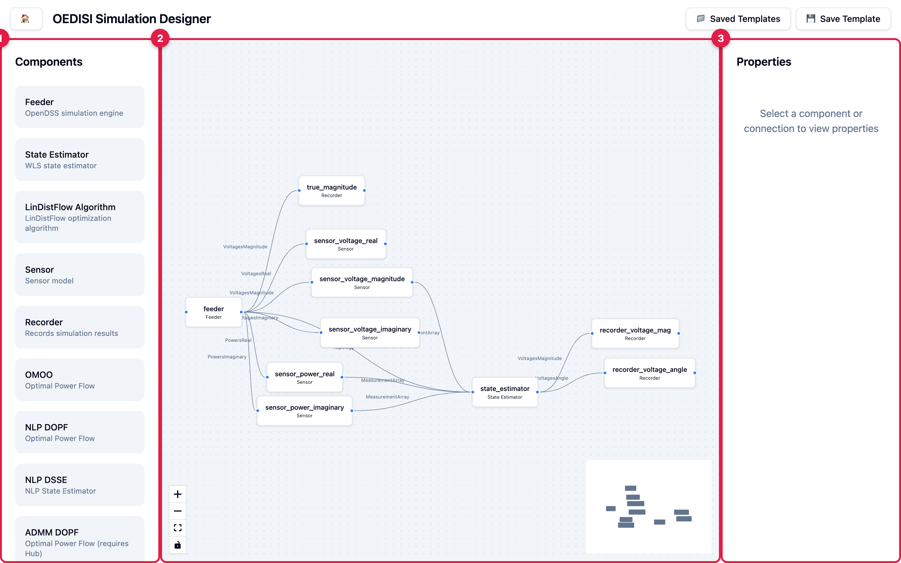
The designer, showing the NLR DSSE example wired up: feeder → sensors → state estimator → recorders.
You build a diagram by dragging components from the palette onto the canvas and connecting their ports:

Drag components from the palette onto the canvas to compose a simulation.
When you connect two nodes, the properties panel lets you pick which typed signal flows
along the edge (for example VoltagesMagnitude from the feeder to a sensor). Use 💾 Save
Template to store your diagram.
Saved templates
Saved Templates lists every simulation you’ve saved. Each card shows the components, the node/connection counts, and actions: Run, Load (open in the designer), Notebook, Download JSON, and Delete.
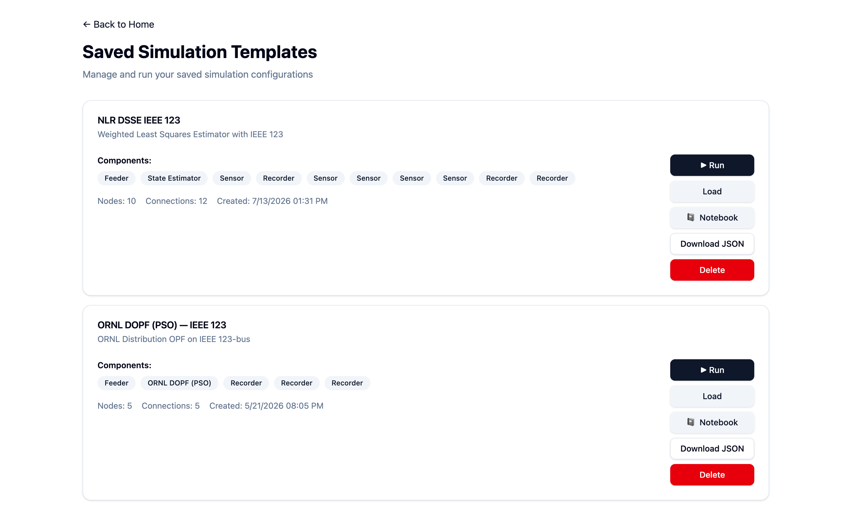
Saved simulation templates.
Runs
Running a template creates a run. The runs list is your history — each row shows the run name, status, and timing.
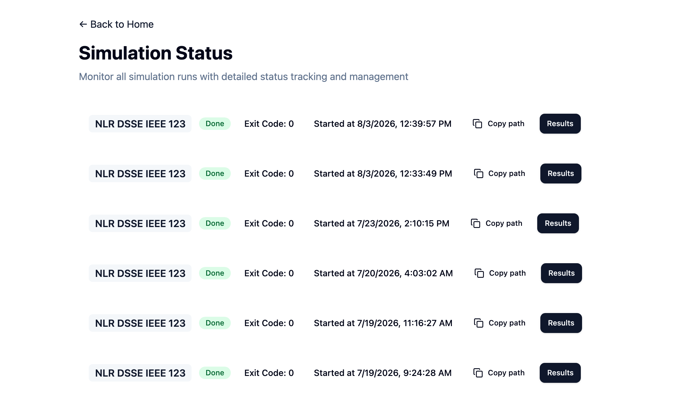
The list of simulation runs.
Run detail
Opening a run shows its live status (running → done/failed), the exit code, and the
per-federate logs. When a run finishes, the Results and Notebook buttons
appear.
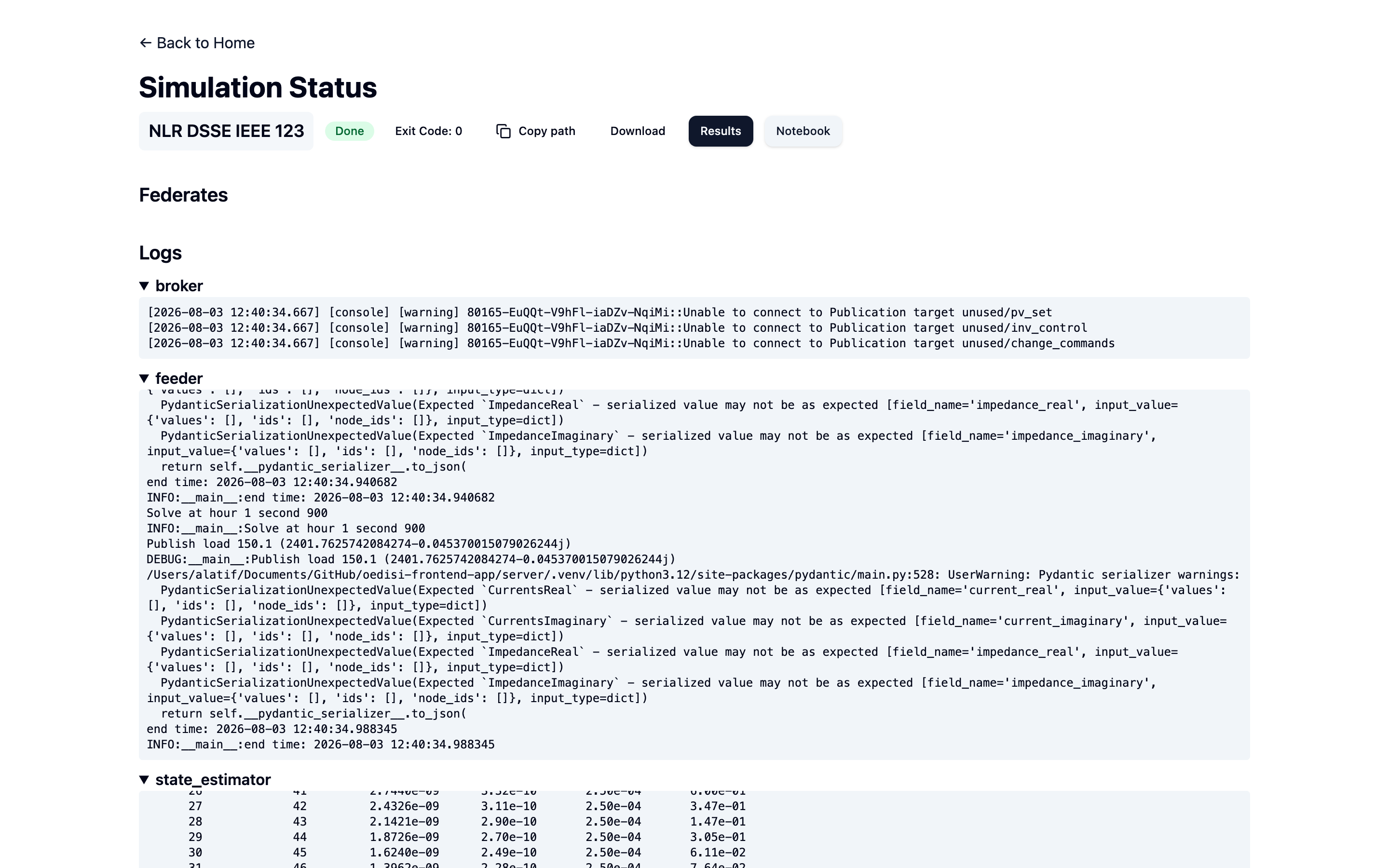
A completed run, with per-federate logs.
Results
The results view plots the data captured by each Recorder. Pick a dataset, scrub through timesteps with the slider, and optionally compare two datasets (for example an estimate against the true values).
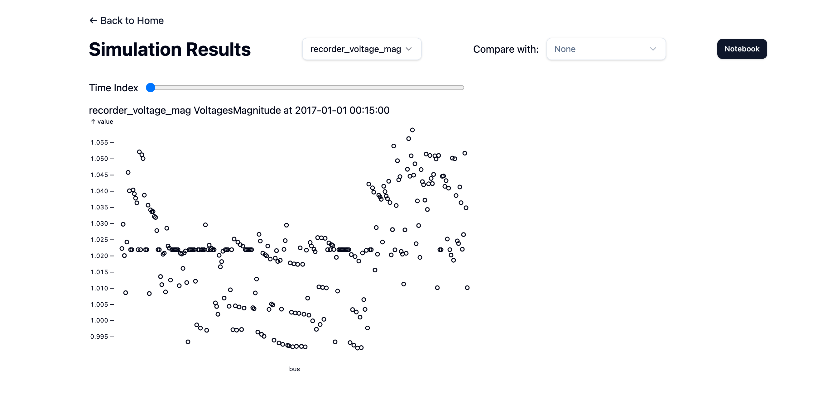
Recorded voltage magnitudes, plotted per bus.
Analysis notebook
For deeper analysis, Notebook opens an embedded JupyterLab pointed at the run’s output
directory. It comes pre-populated with a DATA_DIR and the imports you need, and you can
Save to Template so the analysis travels with every future run.
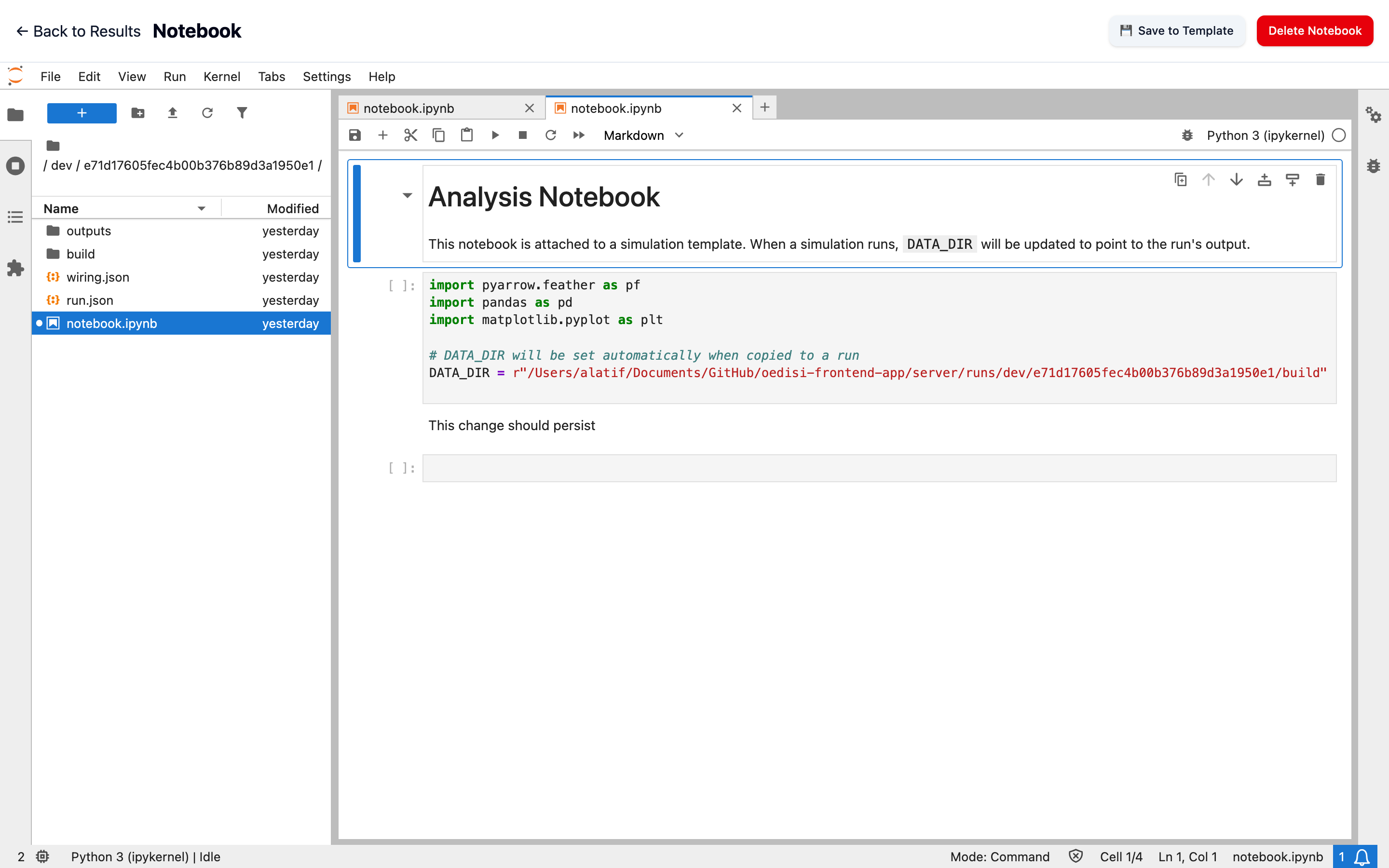
The embedded analysis notebook.
Next steps
Run a template end-to-end.
Reproduce the analysis yourself in the executable results notebook.
Browse the component catalog to see what each block does.